Introduction to reproducible data analysis with R and Quarto
KLI Seminar 2023
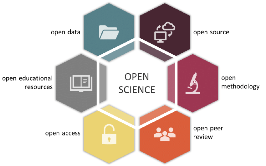
Elements of Open Science
The benefits of Open Science for researchers
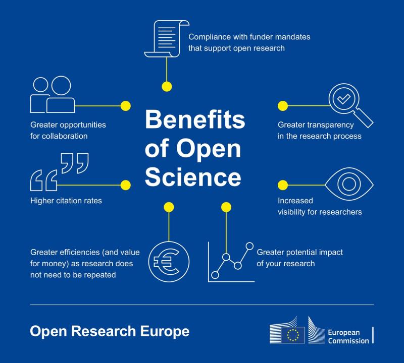
Source: The benefits of Open Science
Source
Output
Source
---
title: "ggplot2 demo"
author: "Norah Jones"
date: "5/22/2021"
format:
html:
fig-width: 8
fig-height: 4
code-fold: true
---
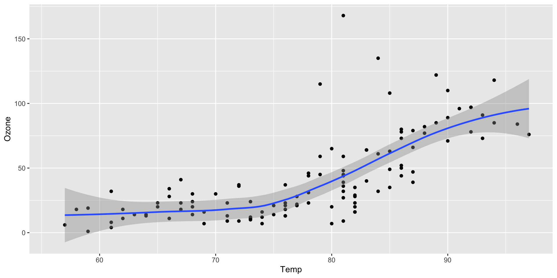
## Air Quality
@fig-airquality further explores the impact of temperature
on ozone level.
```{r}
#| label: fig-airquality
#| fig-cap: Temperature and ozone level.
#| warning: false
library(ggplot2)
ggplot(airquality, aes(Temp, Ozone)) +
geom_point() +
geom_smooth(method = "loess"
)
```Output 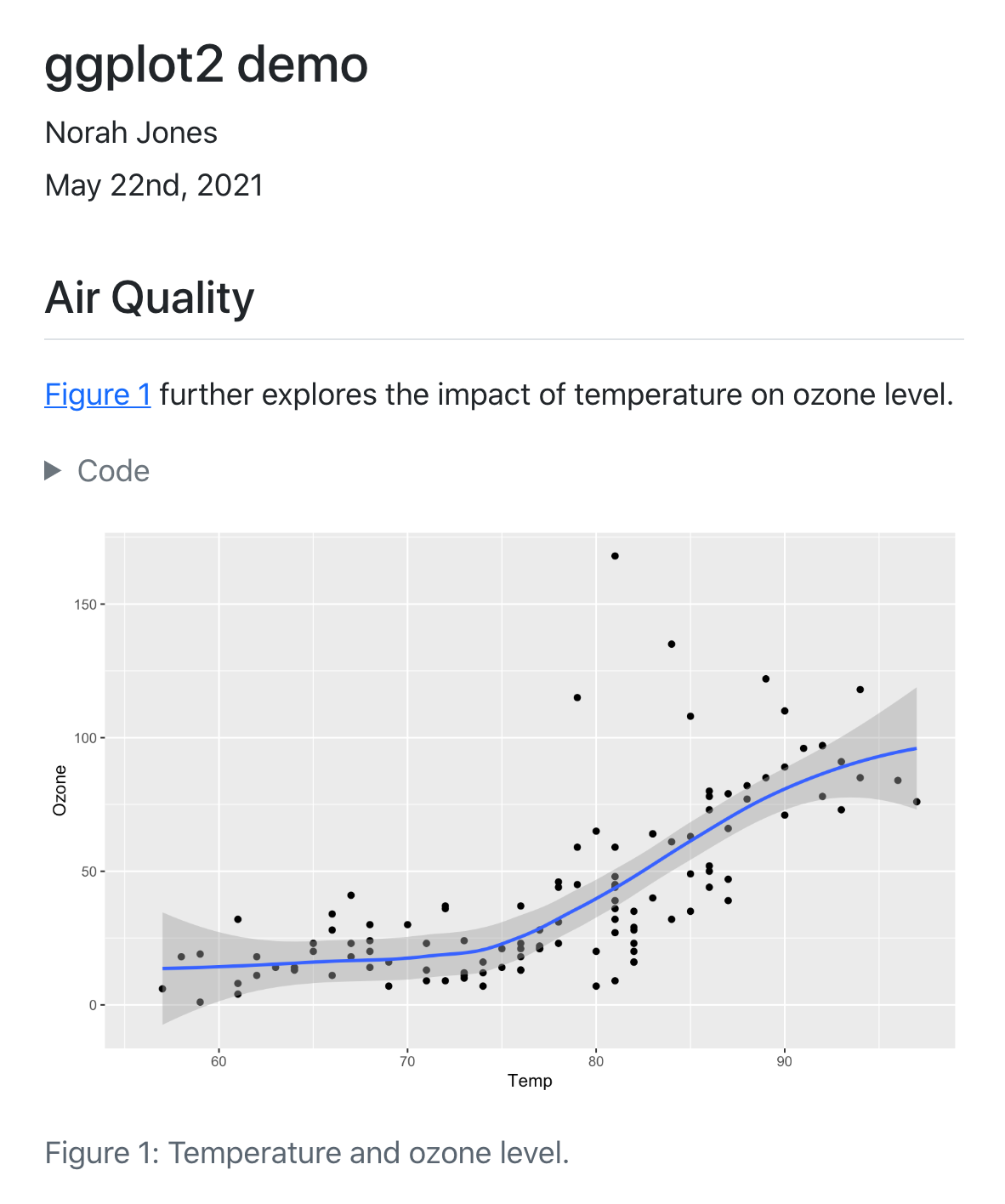
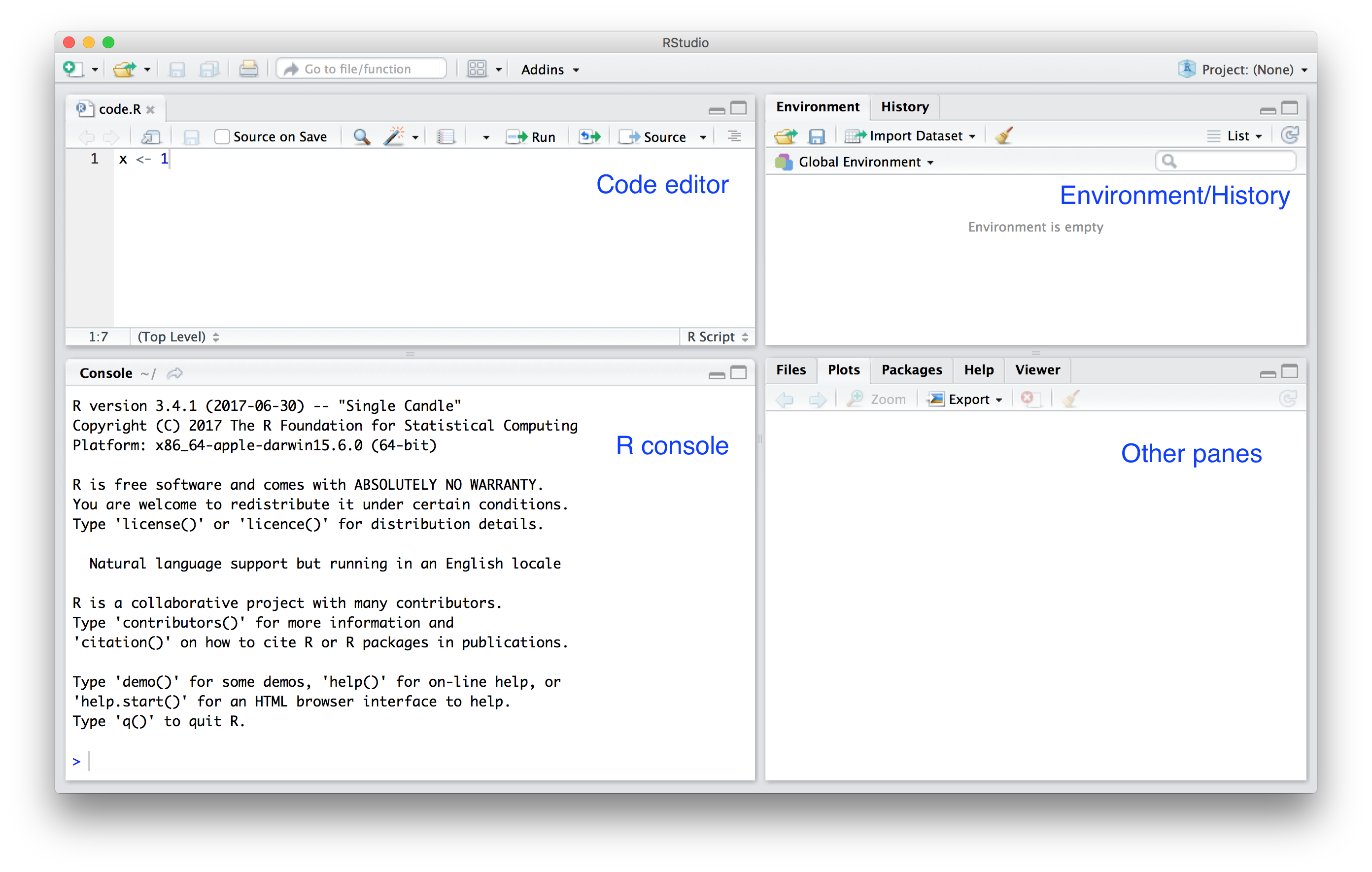
Getting Started with R
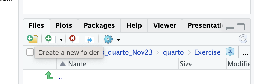
Create a folder for your R project
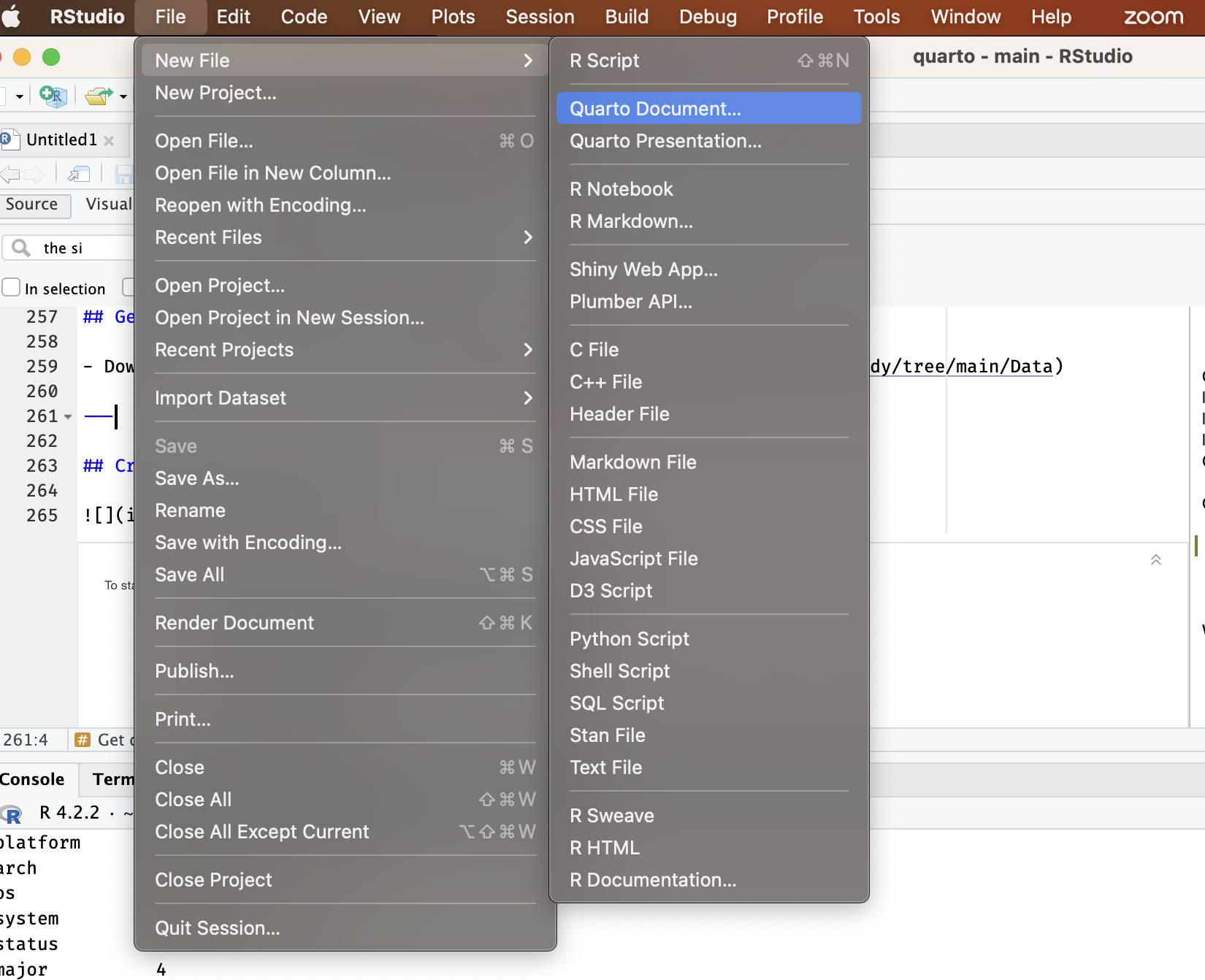
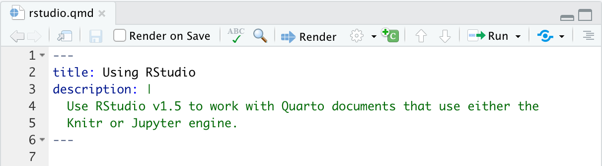
Create a Quarto document (report.qmd)
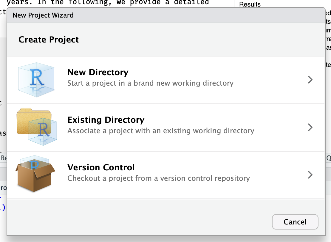
Create an R project
How does Quarto work?
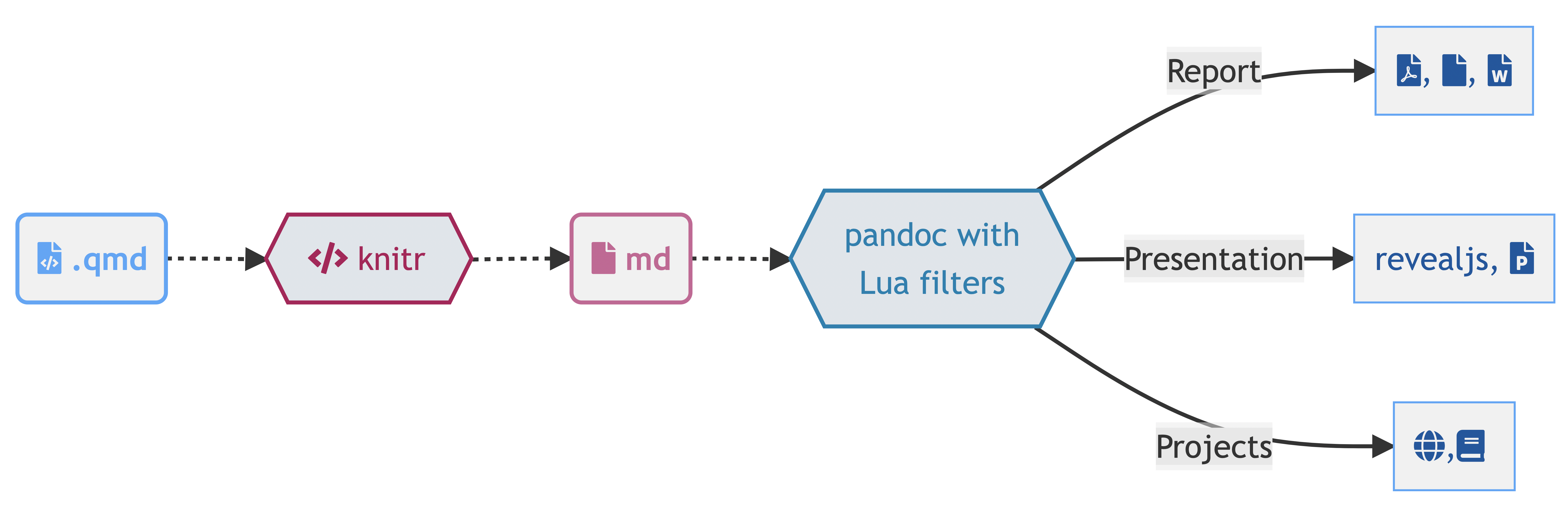
Rendering
- Render button
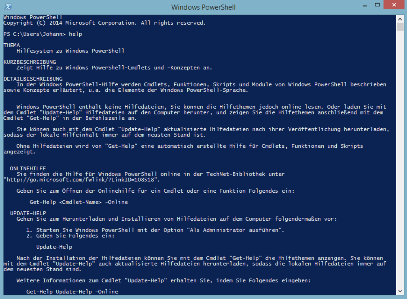
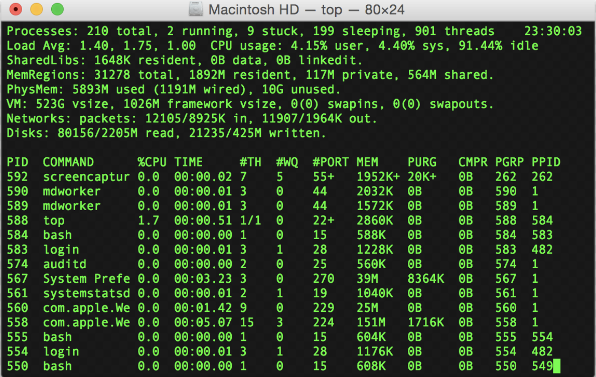
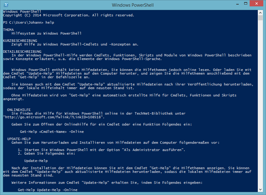
Quick excourse: The Terminal
- Click Start, type PowerShell, right-click Windows PowerShell, and then click Run as administrator
- Click the Launchpad icon in the Dock, type Terminal in the search field, then click Terminal
Quarto workflow
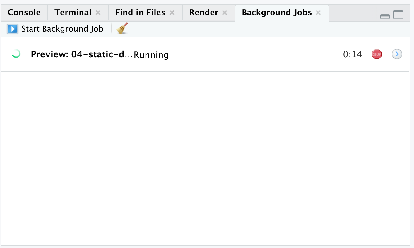
Executing the Quarto Render button in RStudio will call Quarto render in a background job - this will prevent Quarto rendering from cluttering up the R console, and gives you and easy way to stop.
Code
#/media/File:Appleterminal2.png)
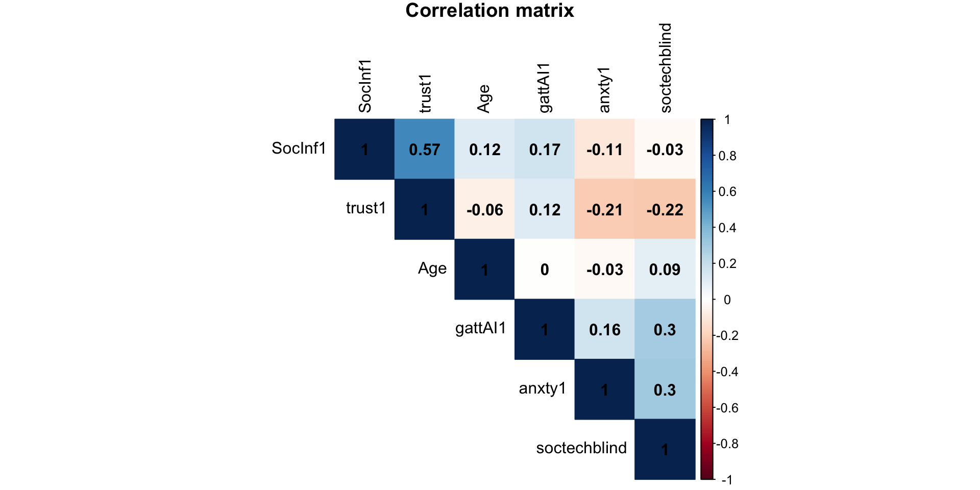
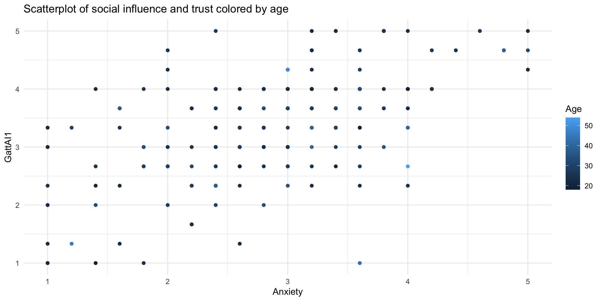
Creating correlation plot
Scatterplot
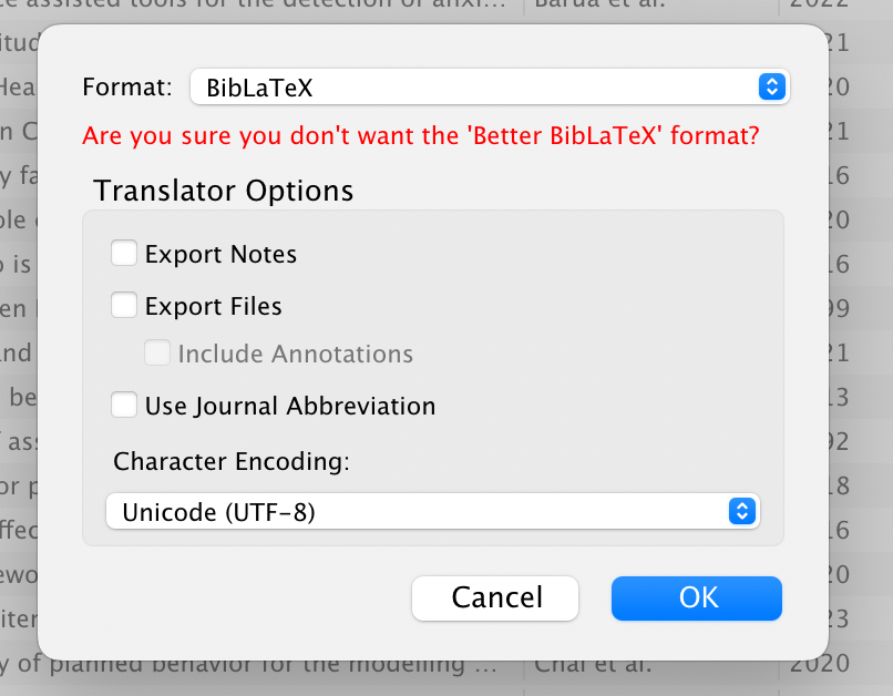
Export the bibliography
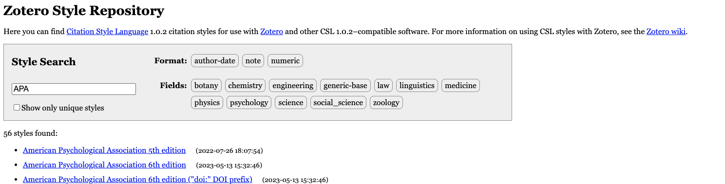
Select a csl style
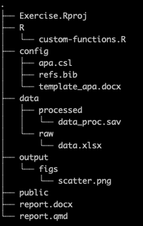
Current folder structure
Back to “report.qmd”
The visual editor and inserting text and citations
Thank you and see you tomorrow!

![]()