Introduction to reproducible data analysis with R and Quarto

Anne-Kathrin Kleine

Schedule

Reproducibility and Open Science

  • The basics of results reproducibility, replicability, and Open Science

Getting Started with R and Quarto

  • Basics of R and Quarto programming
  • Integrating code, text, and output within a Quarto document

Working with data

  • Creating a data analysis project
  • Working with data in R: importing, manipulating, and exporting data
  • Data visualization and data analysis

Workshop Requirements

👉 Open RStudio

Reproducibility and open science

Reproducibility and replicability

Reproducibility

Reproducibility means that research data and code are made available so that others are able to reach the same results as are claimed in scientific outputs.

Closely related is the concept of replicability, the act of repeating a scientific methodology to reach similar conclusions (using other data).

Reproducibility emphasizes re-using original data and methods for verification, while replicability focuses on achieving consistent results with under similar conditions but using new data.

From The Open Science Training Handbook

Open Science for ensuring reproducibility and replicability

Source: The six core principles of Open Science

The benefits of Open Science for behavioral researchers

Source: The benefits of Open Science

Getting Started with R and Quarto

Change your mental model
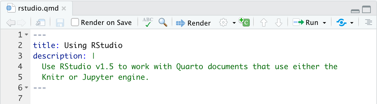
Source

A blank Word document

Output

A blank Word document

Source

---
title: "ggplot2 demo"
author: "Norah Jones"
date: "5/22/2021"
format: 
  html:
    fig-width: 8
    fig-height: 4
    code-fold: true
---

## Air Quality

@fig-airquality further explores the impact of temperature 
  on ozone level.

```{r}
#| label: fig-airquality
#| fig-cap: Temperature and ozone level.
#| warning: false
library(ggplot2)
ggplot(airquality, aes(Temp, Ozone)) + 
  geom_point() + 
  geom_smooth(method = "loess"
)
```

Output

Working with R and RStudio

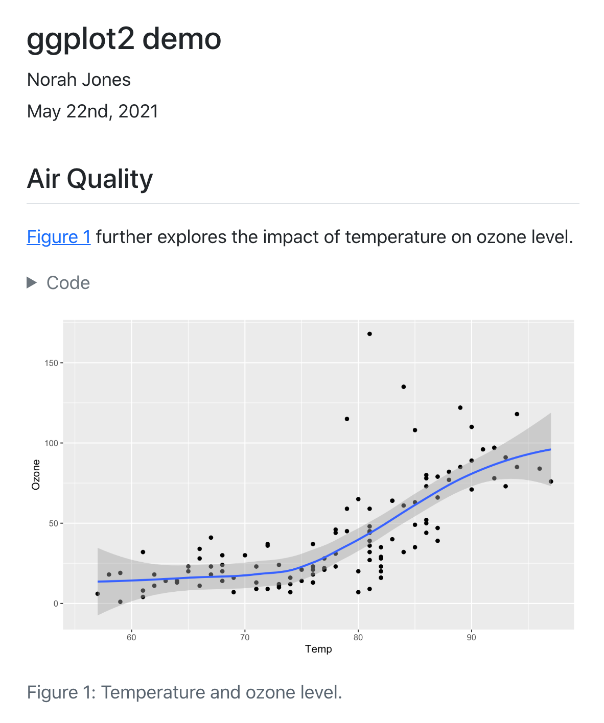
Getting Started with R and RStudio

Create a folder for your R project

Create an R project

R projects

When a project is opened within RStudio the following actions are taken:

🦋 A new R session is started

🐛 The .Rprofile, .RData file, and .Rhistory files in the project’s main directory are loaded

🐝 The current working directory is set to the project directory

🐞 Other RStudio settings (e.g. active tabs, splitter positions, etc.) are restored to where they were the last time the project was closed

Create a Quarto document (report.qmd)

Install some packages

```{r}
#| eval: false
pkg_list <- c("tidyverse", "haven", "flextable", "broom")
install.packages(pkg_list)
```

Quarto

How does Quarto work?

A diagram of how a RMD is turned into output formats via knitr and pandoc

So what is Quarto?

Quarto is a command line interface (CLI) that renders plain text formats (.qmd, .rmd, .md) into static PDF/Word/HTML reports, books, websites, presentations and more

Rendering

A screenshot of the render button in RStudio

For rendering to pdfs see 👉 here

For rendering to word docs see 👉 here

Working with a .qmd

A .qmd is a plain text file

  • Metadata (YAML)
format: html
engine: knitr
  • Code
```{r}
library(dplyr)
mtcars |> 
  group_by(cyl) |> 
  summarize(mean = mean(mpg))
```
  • Text
# Heading 1
This is a sentence with some **bold text**, *italic text* and an 
![image](image.png){fig-alt="Alt text for this image"}.

Metadata: YAML

The YAML header:

influences the final document in different ways. It is placed at the very beginning of the document. The information that it contains can affect the code, content, and the rendering process.

YAML

title: "My Document"
format: 
  html:
    toc: true
    code_folding: 'show'

See more formats and other YAML metadata options here

Markdown

Quarto uses markdown as its underlying document syntax. Markdown is a plain text format that is designed to be easy to write, and, even more importantly, easy to read

Text Formatting

Markdown Syntax Output
*italics* and **bold**
italics and bold
superscript^2^ / subscript~2~
superscript2 / subscript2
~~strikethrough~~
strikethrough
`verbatim code`
verbatim code

Headings

Markdown Syntax Output
# Header 1

Header 1

## Header 2

Header 2

### Header 3

Header 3

#### Header 4

Header 4

Code

```{r}
#| output-location: column
#| fig-cap: Temperature and ozone level.
#| warning: false
library(ggplot2)
ggplot(airquality, aes(Temp, Ozone)) + 
  geom_point() + 
  geom_smooth(method = "loess")
```

Temperature and ozone level.

Working with data

Get data

Reading data in

```{r}
## Read in data
library(readxl)
library(tidyverse)
data <- read_excel("Exercise/data/raw/data.xlsx", col_names = T) # if you created an R project you can use the direct path "data/raw/data.xlsx"
```

Manipulating data

```{r}
# Name correction
names(data) <- gsub("d2priv", "dapriv2", names(data))

# Own function
recode_5 <- function(x) {               
  x * (-1)+6
}

# Use of mutate_at to apply function
data_proc <- data %>%
  mutate_at(vars(matches("gattAI1_3|gattAI1_6|gattAI1_8|gattAI1_9|gattAI1_10|gattAI2_5|gattAI2_9|gattAI2_10")), recode_5)
```

Manipulating data: Creating composites

```{r}
data <- data[ , purrr::map_lgl(data, is.numeric)] %>% # select numeric variables
  select(matches("gattAI1|soctechblind|trust1|anxty1|SocInf1|Age")) # select relevant variables

comp_split <- data %>% sjlabelled::remove_all_labels(.) %>% 
  split.default(sub("_.*", "", names(data))) # creating a list of dataframes, where each dataframe consists of the columns from the original data that shared the same prefix (all characters before the underscore)

comp <- purrr::map(comp_split, ~ rowMeans(.x, na.rm=T)) #calculating the row-wise mean of each data frame in the list `comp_split`, with the output being a new list (`comp`) where each element is a numeric vector of row means from each corresponding data frame in `comp_split`

comp_df <- do.call("cbind", comp) %>% as.data.frame(.) # binding all the elements in the list `comp` into a single data frame, `comp_df`
```

Exporting data

```{r}
library(haven)
write_sav(data_proc, "Exercise/data/processed/data_proc.sav") # if you created an R project you can use the direct path "data/processed/data_proc.sav"
```

The R folder

Storing and sourcing custom functions from the R folder

  • You may store your custom functions in a separate file (e.g., “R/custom-functions.R”) that you may source in your report document (“report.qmd”)

In R/custom-functions.R:

```{r}
# Own function
recode_5 <- function(x) {               
  x * (-1)+6
}
```

In report.qmd:

```{r}
source("Exercise/R/custom-functions.R")
```

Visualisations

Reading in pre-processed data

```{r}
data <- haven::read_sav("Exercise/data/processed/data_proc.sav")
```

Creating a correlation plot

```{r}
cor_matrix <- cor(comp_df[1:6])

corrplot::corrplot(cor_matrix, method="color", type="upper", order="hclust", 
         addCoef.col = "black", # Add correlation coefficient on the plot
         tl.col="black", # Text label color
         tl.srt=90, # Text label rotation
         title="Correlation matrix", mar=c(0,0,1,0))
```

Scatterplot

```{r}
scatter <- ggplot(comp_df, aes(x=SocInf1, y=trust1, color=Age)) +
  geom_point() +
  labs(x="Anxiety", y="GattAI1", color="Age") +
  theme_minimal() +
  ggtitle("Scatterplot of social influence and trust colored by age")
scatter
```

Saving scatterplot

  • Save your scatterplot in an output/figs folder
```{r}
ggsave(filename="Exercise/output/figs/scatter.png", plot=scatter)
```

Review your folder structure

Questions? Remarks?

takk for oppmerksomheten!

@AnneOkk

annekathrinkleine.com

Anne-Kathrin.Kleine@psy.lmu.de